Non-equilibrium

In this section, you will analyze two non-equilibrium properties of proteins, the diffusion of heat and a phenomenon known as temperature echoes. This section requires some knowledge of the principles of statistical physics, but the results of the simulations can be understood intuitively even without a deep understanding of their principles.

Heat Diffusion

For this exercise, you will use the last step of the equilibration of ubiquitin in a water sphere, file ubq_ws_eq.restart.coor. You will use the temperature coupling feature of NAMD to set the temperature of the molecules in the outer layer of the sphere to 200 K, while the rest of the bubble is set to a temperature of 300 K. In this way, you will determine the thermal diffusivity by monitoring change of the system's temperature and comparing it to the theoretical expression.

* 1

Change to this problem's directory in a Terminal window:

cd ../2-6-heat-diff/

In order to use the temperature coupling feature of NAMD, you need to create a file which marks the atoms subject to the temperature coupling. The following lines

tCouple on
tCoupleTemp 200
tCoupleFile ubq_shell.pdb
tCoupleCol B

in the provided configuration file ubq_cooling.conf will enable this feature, and set the atoms coupled to the thermal bath as the ones that have a value of 1.00 in the B column of the ubq_shell.pdb, which you will create below.

* 2

In the VMD TkCon window, navigate to the 2-6-heat-diff/ directory.

cd ../2-6-heat-diff/

3

Load the system into VMD by typing the following in the VMD TkCon window:

mol new ../common/ubq_ws.psf
mol addfile ../1-2-sphere/ubq_ws_eq.restart.coor

4

Select all atoms in the system:

set selALL [atomselect top all]

5

Find the center of the system:

set center [measure center $selALL weight mass]

6

Find $x$, $y$ and $z$ coordinates of the system's center and place their values in the variables xmass, ymass, and zmass:

foreach {xmass ymass zmass} $center { break }

7

Select atoms in the outer layer:

set shellSel [atomselect top "not ( sqr(x-$xmass)
+ sqr(y-$ymass) + sqr(z-$zmass) <= sqr(22) ) "]

8

Set beta parameters of the atoms in this selection to 1.00:

$shellSel set beta 1.00

9

Create the pdb file that marks the atoms in the outer layer by ``1.00'' in the beta column:

$selALL writepdb ubq_shell.pdb

10

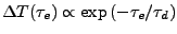
Run the Molecular Dynamics simulation

* 11

If you do not run the simulation yourself, you will need to obtain the data for the temperature from the provided log file. Copy this log file from the directory example-output/.

copy example-output$\backslash$ubq_cooling.log .

If you run the simulation yourself, your log file will be generated by NAMD, and you do not need to copy it.

* 12

Use namdstats.tcl to find out how the system's temperature changes with time. In the VMD TkCon window, type:

source ../2-3-energies/namdstats.tcl
data_time TEMP ubq_cooling.log

The file TEMP.dat will be written with the temperature of the system over time.

* 13

You can now quit VMD.

* 14

In Excel, click File $\rightarrow$ Open$\ldots$, navigate to the directory 2-6-heat-diff/, and choose the file TEMP.dat. Make sure the dropdown menu Files of type is set to All Files.

* 15

When the Text Import Wizard appears, choose Delimited for your file type and click Next. Under the category Delimiters, click Tab. The Data Preview window should show your timestep and temperature data separated into two columns. Click Finish. The timestep and temperature values will appear in Columns A and B, respectively.

* 16

Before plotting the data, we will modify the time units so that they are in units of fs, not timesteps. In cell C1, type the formula =A1*2, click and hold the lower-right corner of C1 and drag down to cell C201. These values are the simulation time in fs.

* 17

Plot the temperature data by clicking Insert $\rightarrow$ Chart$\ldots$, choosing XY (Scatter) as your Chart Type, selecting the last Chart sub-type in the lower-right, and clicking Next.

* 18

In Step 2, click the Series tab, remove any existing series, and click the Add button. Click the red button in the X Values: field, select every data value in Column C (Rows 1-201), and click the red button to complete. Do the same for the Y Values: using the data in Column B. Click Finish.

* 19

Double click on the y-axis and change the Minimum: value to 200. Click OK. Modify the chart further if you wish.

* 20

You will now fit the simulated temperature dependence to the theoretical expression.

* 21

In cell D1, type or copy and paste the formula (make sure it is on one line):

= 200
+66.87*(EXP(-0.0146*E$1*C1) +0.25*EXP(-0.25*0.0146*E$1*C1)
+1/9*EXP(-1/9*0.0146*E$1*C1) +1/16*EXP(-1/16*0.0146*E$1*C1)
+1/25*EXP(-1/25*0.0146*E$1*C1) +1/36*EXP(-1/36*0.0146*E$1*C1)
+1/49*EXP(-1/49*0.0146*E$1*C1) +1/64*EXP(-1/64*0.0146*E$1*C1)
+1/81*EXP(-1/81*0.0146*E$1*C1) +1/100*EXP(-1/100*0.0146*E$1*C1))

The value in cell E1 is the thermal diffusivity, which we will alter to obtain a better fit. Enter an initial guess of 0.03 in cell E1. Then extend the formula in D1 down to cell D201.

* 22

In the chart, right-click on the temperature data and select Source Data$\ldots$. Click the Series tab and add a series with Y Values: of Column D, Rows 1-201. and X Values: of Column C. Click OK.

You may want to change the line weight of your fit by right-clicking the line in your histogram and selecting Format Data Series$\ldots$.

We have our theoretical temperature expression plotted, but the fit is not optimal. If we change thermal diffusivity in cell E1, we will see the fit change. We will now determine the optimal parameters.

* 23

In cell F1, type the formula =(D1-B1)$\wedge$2. Then click and hold the lower-right corner of cell F1 and drag down to row 201 to fill in the error values for each bin.

* 24

Type =sum(F1:F201) into cell G1. This is the total square error for our fit, and it is what we seek to minimize using the Solver tool.

* 25

Click Tools $\rightarrow$ Solver$\ldots$. If that option is not present, you will need to add in the Solver tool by clicking Tools $\rightarrow$ Add Ins$\ldots$ and selecting Solver Add-in from the list.

* 26

In the Solver Parameters window, set the following cell ranges and click Solve:

Set Target Cell: $G$1
Equal To: Min
By Changing Cells: $E$1

Solver will find the thermal diffusivity which optimally fits the temperature expression to our raw temperature data.

Figure 13: Cooling of ubiquitin in a water sphere. The smooth black line shows a non-linear fit of the data to the theoretical expression.

* 27

Multiply the value of the parameter in cell E1 by 0.1 to get the thermal diffusivity in cm$^2$s$^{-1}$. You should get a value of around 0.45$\times10^{-2}$cm$^2$s$^{-1}$. How does your result compare to the thermal diffusivity of water $D=1.4\times10^{-3}$cm$^2$s$^{-1}$?

* 28

Compute the thermal conductivity of the system, $K$, by the following formula: $K=\rho\: c_V D$, where $c_V$ is the specific heat (that was calculated in Section 2.1.5) and $D$ is the thermal diffusivity (assume that the density of the system, $\rho$, is 1 g/mL).

* 29

Save the file you created in Excel if you wish, and close Excel.

Temperature echoes

The motions of atoms in globular proteins (e.g., ubiquitin), referred to as internal dynamics, comprise a wide range of time scales, from high frequency vibrations about their equilibrium positions with periods of several femtoseconds to slow collective motions which require seconds or more, leading to deformations of the entire protein.

The internal dynamics of these proteins on a picosecond time scale (high frequency) can be described as a collection of weakly interacting harmonic oscillators referred to as normal modes. Since normal modes are formed by linear superposition of a large number of individual atomic oscillations, it is not surprising that the internal dynamics of proteins on this time scale has a delocalized character throughout the protein. The situation is similar to the lattice vibrations (phonons) in a crystalline solid. Experimentally, there exist ways to synchronize, through a suitable signal or perturbation, these normal modes, forcing the system in a so-called (phase) coherent state, in which normal modes oscillate in phase. The degree of coherence of the system can be probed with a second signal which through interference with the coherent normal modes may lead to resonances, referred to as echoes, which can be detected experimentally. However, the coherence of atomic motions in proteins decays through non-linear contributions to forces between atoms. This decay develops on a time scale $\tau_d$ which can be probed, e.g., by means of temperature echoes, and can be described by employing MD simulations.

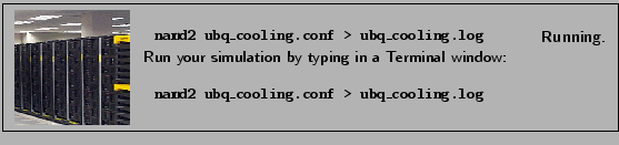
In a temperature echo the coherence of the system is probed by reassigning the same atomic velocities the system had at an earlier time and then looking to an echo in the temperature at time $\tau_e$, as a result of such reassignment. An example is shown in Fig. 14. At time $t_1=0$ the velocities of all atoms in the system are quenched; then, at $t_2=\tau$ the atomic velocities are reassigned again (quenched) to their values at time $t_1=0$. As a result, a temperature echo, i.e., a sharp dip in $T(t)$, is detected at a subsequent time $\tau_e = \tau$ after $t_2$ (i.e., at time $t=2\tau$).

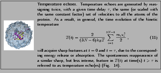
In this section, you will employ MD simulations to generate temperature echoes in ubiquitin by applying the velocity reassignment just described. By modeling ubiquitin as a large collection of weakly interacting harmonic oscillators (normal modes), you will find that:

• the dephasing time $\tau_d$ of the oscillators is about one picosecond;
• the temperature echo can be expressed in terms of the temperature autocorrelation function; and
• the depth $\Delta T(\tau_e)$ of the echoes decay exponentially with the delay time $\tau_e$, i.e., $\Delta T(\tau_e)\propto \exp\left(-\tau_e/\tau_d\right)$, the exponential decay being determined by the dephasing time $\tau_d$.

Figure 14: Temperature quench echo.

First you will generate temperature echoes in MD simulations, and then you will analyze the echoes in the framework of the normal mode approximation.

The phenomenon of temperature echoes has a simple explanation within the normal modes description of a protein. The first velocity reassignment enforces phase coherence for the oscillators. Because of the frequency dispersion of the normal modes (as well as the deviation from the harmonic approximation) the phase coherence of the protein will decay in time with a characteristic dephasing time $\tau_{d} \sim 1$ps. The second velocity reassignment after a delay time $\tau$ is a ``probing signal'' which will test the degree of coherence of the system at the instant of time it was applied. The depth of the echo and the instant of time at which it occurs are quantitative characteristics of the coherence of the internal dynamics of proteins.

In order to generate temperature echoes, one needs to equilibrate ubiquitin at the desired initial temperature $T_0=300$K, e.g., by using the velocity rescaling method. Once the system is equilibrated, the thermostat is removed and all the following simulations are carried out in the microcanonical (NVE) ensemble.

In this section, you will consider two types of temperature echoes. In the first, you will reassign all atomic velocities to zero, and in the second, you will reassign the atomic velocities to a 300 K distribution (the same as the initial temperature of the system) and the second reassignment will be exactly the same as the first.

Temperature quench echo

The temperature quench echo is obtained by resetting to zero the velocity of all atoms of the protein at both times $t_1=0$ and $t_2=\tau$. You should start from the pre-equilibrated protein in vacuum at $T_0=300K$; the required files are located in the common directory.

You need to run the simulations in the microcanonical ensemble (NVE) by using the configuration file equil.conf in the 2-7-echoes/01_equil_NVE directory. The simulation will run for 500 time steps (fs).

* 1

Change to the 2-7-echoes/01_equil_NVE directory in a Terminal window.

Let's take a look at some features in the configuration file. You can read the file using WordPad.

• The simulation takes restart files, i.e., the coordinate file and the velocity file, from an equilibration simulation at $T=300K$.

  # Continuing a job from the restart files
  set inputname      ../common/ubi_equil
  binCoordinates     $inputname.restart.coor
  extendedSystem     $inputname.xsc

• Notice that the temperature line is commented out. The initial temperature is pre-defined by the initial velocities.

  #temperature       $temperature
  binvelocities      $inputname.restart.vel

• Since you are running an NVE simulation, there is no temperature coupling or pressure control.

• As discussed previously, one should use rigidBonds for water in any production simulation since water molecules have been parametrized as rigid molecules. But for the illustration of temperature quench echo, the effect of force field can be negligible. To be simple, the rigidBonds option is turned off.

* 2

Close the configuration file and WordPad.

3

Run the Molecular Dynamics simulation

* 4

If you do not run the simulation yourself, you will need to obtain the data for the temperature from the provided log file. Copy this log file from the directory example-output/.

copy example-output$\backslash$equil.log .

If you run the simulation yourself, your log file will be generated by NAMD, and you do not need to copy it.

* 5

Open VMD by clicking Start $\rightarrow$ Programs $\rightarrow$ VMD.

* 6

Once your job is done, you need to get the temperature data from the output file. In the VMD TkCon window (Extensions $\rightarrow$ Tk Console), navigate to the 2-7-echoes/01_equil_NVE directory if you are not already there.

* 7

Get the temperature data at every timestep using our namdstats.tcl script:

source ../../2-3-energies/namdstats.tcl
data_time TEMP equil.log

This will write the data into the file TEMP.dat.

* 8

You will now calculate the temperature autocorrelation function, which will be used later to analyze the temperature echoes.

* 9

A tcl script has been provided for you to calculate the temperature autocorrelation function. Source the script by typing in the VMD TkCon window:

source auto-corr.tcl

This will put the temperature autocorrelation function in the file auto-corr.dat.

* 10

In Excel, click File $\rightarrow$ Open$\ldots$, navigate to the directory 2-7-echoes/01_equil_NVE/, and choose the file auto-corr.dat. Make sure the dropdown menu Files of type is set to All Files.

* 11

When the Text Import Wizard appears, choose Delimited for your file type and click Next. Under the category Delimiters, click Tab. The Data Preview window should show your time lag and autocorrelation data separated into two columns. Click Finish. The time lag and autocorrelation function values will appear in Columns A and B, respectively.

* 12

Plot the autocorrelation function by clicking Insert $\rightarrow$ Chart$\ldots$, choosing XY (Scatter) as your Chart Type, selecting the last Chart sub-type in the lower-right, and clicking Next. A preview should show that Excel assigned Column A to x-axis and Column B to the y-axis, as we would like. Click Finish.

You will now fit the simulated temperature autocorrelation function to a decaying exponential approximation (see the Science Box).

* 13

In cell C1, type the following formula:

=EXP(-A1/D$1)

The value in cell D1 is the decay (temperature autocorrelation) time, $\tau_0$, and we will alter it to obtain a better fit. Enter an initial guess of 1 in cell D1. Then extend the formula in C1 down to cell C26.

* 14

In the chart, right-click on the temperature autocorrelation function and select Source Data$\ldots$. Click the Series tab and add a new series with Y Values: of Column C, Rows 1-26. and X Values: of Column A. Click OK.

You may want to change the line weight of your functions by right-clicking the lines in your graph and selecting Format Data Series$\ldots$.

We have our approximation to the temperature autocorrelation function plotted, but the fit is not optimal. If we change decay time in cell D1, we will see the fit change. We will now determine the optimal decay time.

* 15

In cell E1, type the formula =(C1-B1)$\wedge$2. Then click and hold the lower-right corner of cell E1 and drag down to row 26 to fill in the error values for each bin.

* 16

Type =sum(E1:E26) into cell F1. This is the total square error for our fit, and it is what we seek to minimize using the Solver tool.

* 17

Click Tools $\rightarrow$ Solver$\ldots$. If that option is not present, you will need to add in the Solver tool by clicking Tools $\rightarrow$ Add Ins$\ldots$ and selecting Solver Add-in from the list.

* 18

In the Solver Parameters window, set the following cell ranges and click Solve:

Set Target Cell: $F$1
Equal To: Min
By Changing Cells: $D$1

Solver will find the decay time which optimally fits the temperature expression to our raw temperature data. This value will be important for a later analysis of your simulations

19

Modify your chart to display a title, axis labels, etc. if you wish.

Figure 15: Temperature autocorrelation function from simulation (black) and a decaying exponential approximation (red).

* 20

Go to the next directory, 02_quencha, by typing in a Terminal window:

cd ..$\backslash$02_quencha

* 21

You will perform the temperature quenching experiment for the value $\tau = 200 fs$. You are going to quench the temperature (set it to zero), and monitor the recovery of the system as it runs for $\tau$ time steps. If you would like to probe other values of $\tau$, you should edit your configuration file echo.conf using WordPad, changing the value of tau:

set tau 200

22

Run the Molecular Dynamics simulation

* 23

If you do not run the simulation yourself, you will need to obtain the data for the temperature from the provided log file. Copy this log file from the directory example-output/.

copy example-output$\backslash$echo.log .

If you run the simulation yourself, your log file will be generated by NAMD, and you do not need to copy it.

* 24

Once your job is done, you need to again get the temperature data from the output file. In the VMD TkCon window, navigate to the 2-7-echoes/02_quencha directory.

* 25

Get the temperature data at every timestep using our namdstats.tcl script, which we have already sourced:

data_time TEMP echo.log

This will write the data into the file TEMP.dat.

Now, you will quench the system for the second time.

* 26

Change to the directory 03_quenchb in a Terminal window.

Note that the configuration file echo.conf indicates that the simulation will run for $3\tau$ steps: run [expr 3*$tau]

27

Run the Molecular Dynamics simulation

* 28

If you do not run the simulation yourself, you will need to obtain the data for the temperature from the provided log file. Copy this log file from the directory example-output/.

copy example-output$\backslash$echo.log .

If you run the simulation yourself, your log file will be generated by NAMD, and you do not need to copy it.

* 29

Again, get the temperature data from the output file. In the VMD TkCon window, navigate to the 2-7-echoes/03_quenchb directory and get the temperature data at every timestep using our namdstats.tcl script:

data_time TEMP echo.log

This will write the data into the file TEMP.dat.

* 30

In a Terminal window, change the name of this output file so as not to confuse it with the others:

move TEMP.dat temp3.dat

* 31

Copy the previous temperature output to this directory, changing their names as you do so:

copy ..$\backslash$01_equil_NVE$\backslash$TEMP.dat .$\backslash$temp1.dat
copy ..$\backslash$02_quencha$\backslash$TEMP.dat .$\backslash$temp2.dat

* 32

Merge the three temperature data files into temp.dat:

type temp1.dat > temp.dat
type temp2.dat » temp.dat
type temp3.dat » temp.dat

You now have the temperature data for the whole temperature quench experiment. You will use Excel to analyze the data.

* 33

In Excel, click File $\rightarrow$ Open$\ldots$, navigate to the directory 2-7-echoes/03_quenchb/, and choose the file temp.dat. Make sure the dropdown menu Files of type is set to All Files.

* 34

When the Text Import Wizard appears, choose Delimited for your file type and click Next. Under the category Delimiters, click Tab. The Data Preview window should show your time and temperature data separated into two columns. Click Finish. The time and temperature values will appear in Columns A and B, respectively.

* 35

Plot the temperature data by clicking Insert $\rightarrow$ Chart$\ldots$, choosing XY (Scatter) as your Chart Type, selecting the last Chart sub-type in the lower-right, and clicking Next. A preview should show that Excel assigned Column A to x-axis and Column B to the y-axis, as we would like. Click Finish.

Note anything unusual? You quenched the temperature twice, and yet you see three drops in temperature! The third one is a temperature echo. See Fig. 16.

Next, you will compare $T(t)$ in the vicinity of the echo ($t=2\tau$) obtained from the MD simulation with the theoretical prediction (14) involving the temperature autocorrelation function obtained also from the MD simulations. The degree of agreement between these two results is a measure of the accuracy of the harmonic approximation.

* 36

You will use a tcl script to calculate the harmonic approximation of the temperature echo, given by Eq. 13. Source the script by typing in the VMD TkCon window:

source harmonic.tcl

This will write the data for the harmonic approximation to the file harmonic.dat.

* 37

In Excel, view the data by clicking Data $\rightarrow$ Get External Data $\rightarrow$ Import Text File$\ldots$, navigate to the directory 2-7-echoes/03_quenchb/, and choose the file harmonic.dat. Make sure the dropdown menu Files of type is set to All Files.

* 38

When the Text Import Wizard appears, choose Delimited for your file type and click Next. Under the category Delimiters, click Tab. The Data Preview window should show your time and temperature approximation data separated into two columns. Click Finish. When the Import Data window appears, select Existing worksheet: and click cell C1 when asked where you want to put the data. The time and temperature values will appear in Columns C and D, respectively.

* 39

Plot the harmonic approximation data by right-clicking on your existing graph and selecting Source Data$\ldots$. Click the Series tab and add a series with X Values: of Column C, Rows 1-601. and Y Values: of Column D, Rows 1-601. Click OK.

* 40

You need to find the depth of the echo. Do this by looking at Column B or by entering the following formula into cell E1:

= 75 - MIN(B800:B1000)

75 is the average temperature after the second quench, and it corresponds to 1/4 of the initial temperature $T_0$=300K. Note that this formula is designed knowing the echo is between 800 and 1000 fs.

Figure 16: A comparison of the simulation and the expression from harmonic approximation at the vicinity of the echo.

You have calculated the echo depth for a particular value of the delay time $\tau = 200 fs$. You may wish to repeat the experiment using other values of $\tau$ (100-800 fs). (You must alter the harmonic.tcl script.) If this is done and the data is plotted and fitted to a single exponential $\exp(-\tau/\tau_{d})$, one obtains the so-called dephasing time $\tau_{d}$, which is an inherent property of the system.

Velocity replacement echo

Here you will generate a temperature echo by replacing the velocities of the atoms at time $t_2$ with the ones you assign to them at time $t_1$. Moreover, by choosing these velocities according to the Maxwell-Boltzmann distribution corresponding to $T_0=300$K, i.e., the temperature of the equilibrated system ($t<0$), there will be no discontinuities (jumps) in $T(t)$ at $t_1$ and $t_2$, yet you will observe a temperature echo at a later time, i.e., a sharp dip in the temperature at time $t=\tau+\tau_e$. Your goal is to determine $\tau_e$ and the depth $\Delta T$ of the echo. To this end, you will need to follow a similar procedure to the one in the previous exercise.

* 41

In a Terminal window, navigate to the directory 04_consta.

* 42

Reassign the velocities at $t_1$ according to a Maxwell-Boltzmann distribution for a temperature $T_1=300K$, saving the reassigned velocities to a file 300.vel. In order to do this, the following is added to the end of your configuration file echo.conf:

run 0
output 300

These settings will not really run a simulation, but will assign initial velocities with the desired distribution and save them to 300.vel. Following these, the normal run command is used to perform a simulation for tau time steps:

run $tau

43

Run the Molecular Dynamics simulation

* 44

If you do not run the simulation yourself, you will need to obtain the data for the temperature from the provided log file. Copy this log file from the directory example-output/.

copy example-output$\backslash$echo.log .

If you run the simulation yourself, your log file will be generated by NAMD, and you do not need to copy it.

* 45

In the VMD TkCon window, navigate to the 04_consta directory. Use the script namdstats.tcl to get the temperature data as before and put it in the file TEMP.dat. Note that at the beginning there is a duplicate entry for the first time step. You should delete one of these using your text editor:

500 300.5656
500 300.5656
501 301.0253
502 302.5395
...

* 46

In a Terminal window, go to the directory 05_constb.

47

For this simulation, you should use the file 300.vel you generated before as the velocity restart file. This is included in the configuration file echo.conf as:

velocities ../04_consta/300.vel

This will reassign the velocities to the exact same distribution they had at the beginning of the previous simulation. This simulation will run for 3$\tau$ time steps.

48

Run the Molecular Dynamics simulation

* 49

If you do not run the simulation yourself, you will need to obtain the data for the temperature from the provided log file. Copy this log file from the directory example-output/.

copy example-output$\backslash$echo.log .

If you run the simulation yourself, your log file will be generated by NAMD, and you do not need to copy it.

* 50

Again, in the VMD TkCon window, navigate to the 05_constb directory and use the script namdstats.tcl to output the temperature data to the file TEMP.dat.

* 51

In a Terminal window, change the name of this output file and copy the other temperature file to this directory:

move TEMP.dat temp2.dat
copy ..$\backslash$04_consta$\backslash$TEMP.dat .$\backslash$temp1.dat

* 52

Merge the two temperature data files into temp.dat:

type temp1.dat > temp.dat
type temp2.dat » temp.dat

* 53

Note that there are now two temperature values at 700 fs. You should open the file temp.dat with your text editor and delete one.

* 54

Use Excel to plot the temperature data and observe the temperature echo as you did before.

* 55

Locate the position of the echo and measure its depth. This time, the depth is measured by:

Echo depth = 300 - Minimum Temperature

* 56

Compare your result with the pre-made results stored in the directory example-output for $\tau = 200$ fs. How would you explain your findings?

* 57

You can now close VMD and Excel.