Next: Constant Force Pulling
Up: Steered Molecular Dynamics
Previous: Removing Water Molecules
Subsections
In this first simulation you will stretch ubiquitin through the constant velocity pulling
method.
In this type of simulation the SMD atom is attached to a dummy
atom via a virtual spring. This dummy atom is moved at constant velocity
and then the force between both is measured using:
where:
 Potential energy.
 Spring constant.
 Pulling velocity.
 Time.
Time.
-
 Actual position of the SMD atom.
-
 Initial position of the SMD atom.
-
 Direction of pulling.
Figure 17:
Pulling in a one-dimensional case. The dummy atom is colored red, and the SMD atom blue. As the dummy atom moves at constant velocity the SMD atom experiences a force that depends linearly on the distance between both atoms.
![\begin{figure}\begin{center}
\includegraphics[scale=0.5]{pictures/tut_unit03_001c}
\end{center}
\end{figure}](img168.png) |
NAMD uses a column of a pdb file to determine which atoms are fixed:
all atoms with a value of 1 (or a number different of 0) in a predetermined column
will be fixed; atoms with a value of 0 in the same column
will not be affected. Here you will use the B column of the pdb file to designate fixed atoms. Now you need to build the respective pdb file using VMD.
- 1
- Choose the File
 New Molecule... menu item and using the Browse
 and Load buttons load the file
common/ubq.psf that you created in the first unit for
ubiquitin in vacuum. (If you did not succeed in generating this file in unit 1, look for common/example-output/ubq.psf)
and Load buttons load the file
common/ubq.psf that you created in the first unit for
ubiquitin in vacuum. (If you did not succeed in generating this file in unit 1, look for common/example-output/ubq.psf)
- 2
- In the Molecule File Browser window, use the Browse... and the Load buttons load the file common/ubq_ww_eq.pdb into your psf file. Be certain that the Load files for: field says 1:ubq.psf. When you are done, close the Molecule File Browser window. The equilibrated ubiquitin without water is now available in VMD.
- 3
- In the VMD TkCon window, write the following command:
set allatoms [atomselect top all]
|
|
This creates a selection called allatoms which contains all atoms!
- 4
- Type $allatoms set beta 0. In this way you set the B column of all atoms equal to 0.
- 5
- Type set fixedatom [atomselect top "resid 1 and name CA"].
This creates a selection that contains the fixed atom, namely the C
 atom of
the first residue.
atom of
the first residue.
- 6
- Type $fixedatom set beta 1. This sets the value of the B column for the fixed atom to 1
and, therefore, NAMD will keep this atom now fixed.
Likewise, NAMD uses another column of a pdb file to set which atom
is to be pulled (SMD atom). For this purpose it uses the occupancy column of the pdb file.
- 7
- Type $allatoms set occupancy 0, so the occupancy column of every atom becomes 0.
- 8
- Type set smdatom [atomselect top "resid 76 and name CA"].
The smdatom selection you created contains the C atom of the last residue.
- 9
- Type $smdatom set occupancy 1. Now, the occupancy column of the smdatom selection
is 1, and NAMD will pull this atom.
- 10
- Finally, type $allatoms writepdb common/ubq_ww_eq.ref. This will write a file in pdb format that contains
all the atoms with the updated B and occupancy columns. Keep VMD opened.
- 11
- Take a look at the pdb file you have just created. Open a new Terminal window, and change the directory to namd-tutorial-files, by typing cd Workshop/namd-tutorial-files.
- 12
- Open the file by typing VMD text editor common/ubq_ww_eq.ref.
Find the line or row that corresponds to the C atom as shown in Fig. 18 (a) for the methionine (b) residue number 1 (c) or N terminus. In that line you should be able to see how the B column was switched to 1 (e), while the B column for all the other atoms is 0 (d).
Figure 18:
Snapshot of the file ubq_ww_eq.ref showing the fixed atom row.
![\begin{figure}\begin{center}
\par
\par
\latex{
\includegraphics[scale=0.5]{pictures/tut_unit03_002}
}
\end{center}
\end{figure}](img171.png) |
- 13
- The file you just created (common/ubq_ww_eq.ref) also contains the appropriate information required by NAMD
to identify the SMD atom. Again, check this by finding the row or line that corresponds
to the C
 atom as shown in Fig. 19 (a) for the glycine (b) residue number 76 (c) or C terminus.
This atom, that should have occupancy 1 (e), will be pulled in the simulation.
atom as shown in Fig. 19 (a) for the glycine (b) residue number 76 (c) or C terminus.
This atom, that should have occupancy 1 (e), will be pulled in the simulation.
Figure 19:
Snapshot of the file ubq_ww_eq.ref showing the SMD atom row.
![\begin{figure}\begin{center}
\par
\par
\latex{
\includegraphics[scale=0.5]{pictures/tut_unit03_003}
}
\end{center}
\end{figure}](img173.png) |
- 14
- When you are done with the comparison of your file with Figs. 18 and 19,
close VMD text editor.
Note that coordinates (columns 7, 8, and 9) in your file will not necessarily
match the ones shown in the figures because initial velocities in the equilibration were chosen randomly.
Now that you have defined the fixed and SMD atom, you need to specify the direction in which the pulling will be performed. This
is determined by the direction of the vector that links the fixed and the SMD atoms.
- 15
- Type the following commands in the VMD TkCon window:
| set smdpos [lindex [$smdatom get {x y z}] 0] |
|
| set fixedpos [lindex [$fixedatom get {x y z}] 0] |
|
vecnorm [vecsub $smdpos $fixedpos]
|
|
This gives you three numbers that are the  ,
,  , and
, and  - components of the normalized direction between the fixed and the SMD atom!
Keep these
- components of the normalized direction between the fixed and the SMD atom!
Keep these  ,
,  and
and  saved for the next section.
In the provided example (look at Figs. 18 and 19), the result is:

- 16
- Delete the current molecule by choosing the Molecule Delete Molecule menu item and keep VMD opened.
Now you have one of the files required for the intended SMD simulation,
namely common/ubq_ww_eq.ref. The next step is to create the NAMD
configuration file or modify the provided template. Exercise care at this
stage and check for misspelling of names or commands.
- 1
- Be sure that the current directory in the Terminal window is
namd-tutorial-files.
- 2
- Copy the file common/sample.conf to the directory 3-1-pullcv and rename it by typing cp common/sample.conf 3-1-pullcv/ubq_ww_pcv.conf.
- 3
- Open the configuration file using VMD text editor by typing
VMD text editor 3-1-pullcv/ubq_ww_pcv.conf.
- 4
- As a job description you may write
# N- C- Termini Constant Velocity Pulling
|
|
Note that this is just a comment line.
- 5
- In the Adjustable Parameters section you need to change:
| structure mypsf.psf |
|
structure ../common/ubq.psf |
| coordinates mypdb.pdb |
|
coordinates ../common/ubq_ww_eq.pdb |
| outputName myoutput |
|
outputName ubq_ww_pcv |
In this way you are using the equilibrated protein without water in your upcoming simulation. The output files of your simulation will have the prefix ubq_ww_pcv in their names.
- 6
- In the Input section change:
| parameters par_all27_prot_lipid.inp |
|
parameters ../common/par_all27_prot_lipid.inp
|
|
There is no need to modify the Periodic Boundary Conditions,
Force Field Parameters, Integrator Parameters or PME sections (The latter is disabled since you are not using periodic boundary conditions).
- 7
- The temperature control should be disabled in order to disturb the movement of the atoms as little as possible.
Switch off the Constant Temperature Control by changing:
| langevin on |
|
langevin off |
- 8
- Again, there is no need to modify Constant Pressure Control and IMD Settings since they will not be used. However, you have to enable the Fixed Atoms Constraint by changing the following lines:
| if {0} { |
|
if {1} { |
| fixedAtomsFile myfixedatoms.pdb |
|
fixedAtomsFile |
| |
|
../common/ubq_ww_eq.ref |
NAMD will keep fixed the atoms which have a B value of 1 in the file ubq_ww_eq.ref.
- 9
- In the Extra Parameters section add the following lines:
| SMD |
on |
| SMDFile |
../common/ubq_ww_eq.ref |
| SMDk |
7 |
| SMDVel |
0.005 |
With these configuration file modifications, NAMD will pull atoms which have occupancy 1 in the
file ubq_ww_eq.ref. The virtual spring between the dummy
atom and the SMD atom will have a spring constant of 7 kcal/mol/Å ,
where 1 kcal/mol = 69.479 pN Å. The pulling will be performed
at a constant velocity of 0.005 Å/timestep, equivalent to 2.5 Å/ps in
the present case where the time step is 2 femtoseconds.
,
where 1 kcal/mol = 69.479 pN Å. The pulling will be performed
at a constant velocity of 0.005 Å/timestep, equivalent to 2.5 Å/ps in
the present case where the time step is 2 femtoseconds.
- 10
- In the Extra Parameters section you need to write also the
direction of pulling by adding the following line:
Where , and should be replaced by the
coordinates you calculated at the end of section 3.2.1. (In our example,
the direction is  ,
,  ,
,  .)
.)
- 11
- In the same section, set the frequency in time steps with which the current SMD data values will be printed out by typing:
- 12
- Finally, in the Execution Script section of your configuration file be sure that the minimization is disabled and change the number of time steps of your simulation by replacing:
| run 50000 |
|
run 20000 |
This is equivalent to 40 ps (and the simulation should not take more than 20 minutes).
- 13
- Now your configuration file is ready. SAVE IT and close your text editor.
All the files you need to launch your simulation are now ready. You should have a file called ubq_ww_pcv.conf in the 3-1-pullcv directory and files:
- ubq.psf
- ubq_ww_eq.pdb
- ubq_ww_eq.ref
- par_all27_prot_lipid.inp
in the common directory. In case that you have not generated these files you can use prepared files available in the
directories 3-1-pullcf/example-output and common/example-output.
- 1
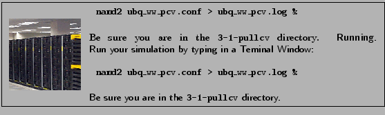
- Check that you actually have these files in the respective directories and change to directory 3-1-pullcv to run the simulation.
While your simulation is running, some files will be created (as you already learned in Unit 1). The only difference in this case is that in the output file (ubq_ww_pcv.log) you will find specific information about the SMD atom and the applied force.
- The additional output line
starts with the word SMD in the first column as shown in Fig. 20 (a).
- The second column (b) is the number of timesteps.
- The third, fourth, and fifth columns (c) are the coordinates of the SMD atom.
- The last three columns (d) are the components of the current force applied to the SMD atom in pN.
Figure 20:
Typical output of a SMD simulation
![\begin{figure}\begin{center}
\par
\par
\latex{
\includegraphics[scale=0.5]{pictures/tut_unit03_004}
}
\end{center}
\end{figure}](img194.png) |
Since the simulation will take some time, the analysis of the complete output will be explained in section 3.4. Thus, while you wait for the result you can set up your Constant Force simulation.
Next: Constant Force Pulling
Up: Steered Molecular Dynamics
Previous: Removing Water Molecules
namd@ks.uiuc.edu
![$\displaystyle \frac{1}{2}k[vt-(\vec{r}-\vec{r}_0)\cdot\vec{n}]^2$](img160.png)
![\framebox[\textwidth]{
\begin{minipage}{.2\textwidth}
\includegraphics[width=2...
...oms is attached to
the dummy atom through the virtual spring.}
\end{minipage} }](img169.png)
![\framebox[\textwidth]{
\begin{minipage}{.2\textwidth}
\includegraphics[width=2...
...nt to use (X, Y, Z, O or B) with the parameter fixedAtomsCol.}
\end{minipage} }](img175.png)